Basic Probability

Mathematics (Core) revision notes · Cambridge (CIE) · 0580 · Core

Back Flashcards

1. The probability scale and its vocabulary

Measuring likelihood

Every probability is a number from 0 to 1, where 0 means impossible and 1 means certain
Halfway, at 0.5, the outcome is as likely to happen as not
Answers may be given as a fraction, a decimal or a percentage, and all three are accepted, but a ratio such as 7 : 20 or words such as "7 out of 20" can lose the mark
Where the question does not specify, a fraction is usually safest, since it stays exact
A probability outside 0 to 1 is always an error, so check any answer above 1 or below 0

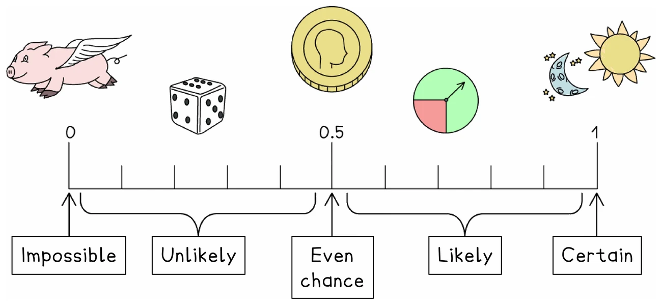
A probability scale running from 0 to 1 with words underneath: impossible at 0, unlikely between 0 and 0.5, even chance at 0.5, likely between 0.5 and 1, and certain at 1, with a flying pig at the impossible end, a dice above the unlikely side, a coin at even chance, a spinner that is three-quarters green above the likely side, and a moon beside the sun at the certain end — Source: Basic probability by Save My Exams

The words that carry meaning

An experiment is repeated to produce results, and each repeat is a trial
An outcome is one possible result; an event may be a single outcome or several of them taken together
The sample space collects every possible outcome, and is usually set out either as a list or in a table
Something is fair when every outcome is equally likely, and biased when they are not
Picking at random means every item has the same chance of being chosen

2. Calculating a probability

Equally likely outcomes

With equally likely outcomes, count how many produce the event and divide that count by how many outcomes there are altogether
Count the total carefully, since it is the denominator of everything that follows
- A bag holds 40 counters of which 14 are red, so the probability of drawing a red one is 14 ÷ 40, which simplifies to 7/20
Simplifying is not required unless the question asks for the simplest form: the mark schemes accept any equivalent fraction, such as 14/40
Information may come from a table, a graph or a Venn diagram rather than from a sentence

Probabilities that must add to 1

Every outcome of an experiment together accounts for the whole of the probability, so they add to 1
A table with one probability missing is completed by subtracting the others from 1
The event not happening takes up whatever is left, so for an event A, the probability of A not happening is 1 − the probability of A happening, written P(not A) = 1 − P(A) for short
- Where a train has a 0.28 chance of being late, the chance of it not being late is 1 − 0.28 = 0.72
Events that can never occur together are mutually exclusive, and for those the chance of one or the other is simply the sum of the two
An event and its complement are always mutually exclusive, which is why they add to 1

Exam tip

Write the subtraction from 1

When a probability table has a gap, the subtraction from 1, such as 1 − (0.3 + 0.25), earns a method mark on its own, even if a later step slips, so write it as a line first. If two gaps are linked, as in "green is twice as likely as yellow", share the 0.45 that is left, not 1: green takes 2 parts and yellow 1, so yellow is 0.45 ÷ 3 = 0.15 and green 0.3.

Worked example

Completing a probability table

A bag holds beads that are red, blue, green or yellow. A bead is taken at random. The table shows the probabilities of red, blue and green. Find the probability of yellow, and the probability of taking a green or a yellow bead.

Colour	red	blue	green	yellow
Probability	0.35	0.2	0.15

Solution:

The four probabilities together must come to 1
The three given ones total 0.35 + 0.2 + 0.15 = 0.7
So the probability of yellow is 1 − 0.7 = 0.3
One bead cannot be both green and yellow, so those events are mutually exclusive and their probabilities add
P(green or yellow) = 0.15 + 0.3 = 0.45

3. Listing the outcomes

Sample space diagrams

Where two things happen together, such as two dice or a dice and a coin, a table lays out every combination
Put one experiment's outcomes along the top and the other's down the side, then fill in the result of each pair
The number of cells is the total number of outcomes, and counting the ones that satisfy the event gives the numerator
Two ordinary dice give 6 × 6 = 36 outcomes, and a systematic table makes them impossible to miscount
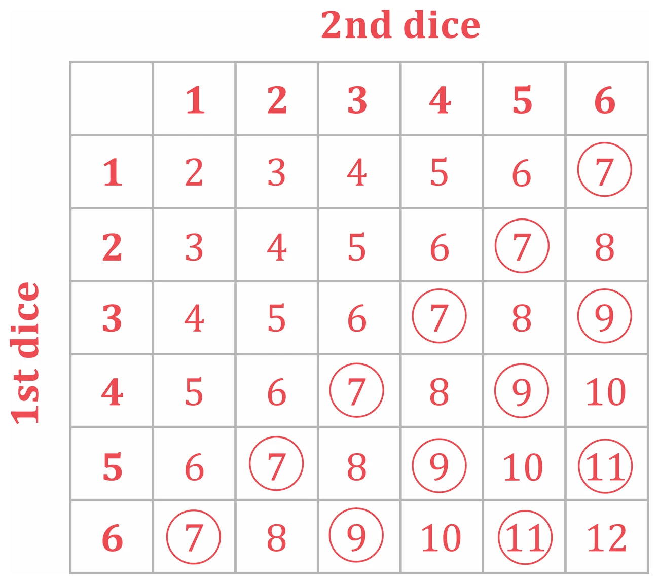
- A total of 9 arises from (3, 6), (4, 5), (5, 4) and (6, 3), so its probability is 4 ÷ 36 = 1/9

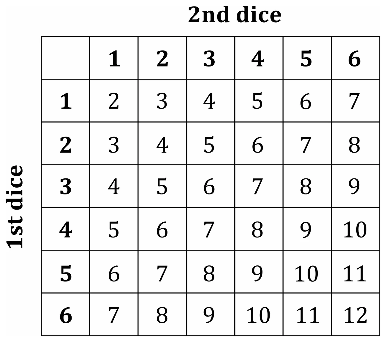
A 6 by 6 table with the first dice down the side and the second across the top, each of the 36 cells holding the total of that pair, so the totals run from 2 in the top left corner to 12 in the bottom right — Source: Possibility Diagrams by Save My Exams

Even if the dice look identical, they are two separate dice, so (3, 6) and (6, 3) are different outcomes and both are counted
Filling the whole table before counting is faster than trying to spot the successes directly

The same table of dice totals with every odd total above 6 circled: six 7s, four 9s and two 11s, twelve circled cells out of the 36, which is how the numerator of the probability is counted — Source: Possibility Diagrams by Save My Exams

Worked example

Reading a probability off a sample space

Two ordinary dice are rolled and their scores added. Find the probability that the total is 10 or more.

Solution:

Each die has 6 faces, so the sample space has 6 × 6 = 36 equally likely outcomes
List the pairs giving a total of 10 or more, taking them in order so none is missed
Total 10: (4, 6), (5, 5), (6, 4)
Total 11: (5, 6), (6, 5)
Total 12: (6, 6)
That is 6 successful outcomes out of 36
P(total ⩾ 10) = 6/36 = 1/6
Even if the dice look identical, they are two separate dice, so (4, 6) and (6, 4) are two different outcomes, not one

4. Relative and expected frequency

Relative frequency

Some probabilities cannot be worked out in advance, so they are estimated from an experiment instead
Relative frequency = number of successes ÷ total number of trials
It is only an estimate, and the more trials are run the closer it should get to the true probability
Comparing a relative frequency with the theoretical probability is how a spinner or dice is judged fair or biased
- A fair six-sided dice should give a five about 1/6 of the time, roughly 0.167
- Rolling 300 times and getting 48 fives gives a relative frequency of 48 ÷ 300 = 0.16, close enough to suggest the dice is fair
- A relative frequency far from the theoretical value suggests bias

Expected frequency

Going the other way, a known probability predicts how often something should happen in a given number of trials
Expected frequency = probability × number of trials
The answer is a prediction rather than a guarantee, so the actual number will usually differ a little
A non-whole answer is acceptable, since an expected frequency is an average rather than a count
- With a probability of 0.15 over 400 trials, the expected frequency is 0.15 × 400 = 60

Worked example

Relative frequency and expected frequency together

A spinner has five equal sections numbered 1 to 5. In an experiment it is spun 200 times and lands on 4 on 32 occasions. Find the relative frequency of landing on 4, say whether the spinner appears to be fair, and find the expected number of 4s in 500 spins of a fair spinner.

Solution:

Relative frequency = 32 ÷ 200 = 0.16
For a fair five-section spinner the theoretical probability is 1 ÷ 5 = 0.2
0.16 is reasonably close to 0.2, so on this evidence the spinner appears roughly fair, though more trials would give a better test
For a fair spinner, expected frequency = probability × number of trials
Expected number of 4s = 0.2 × 500 = 100
Had the question asked how many 4s to expect in 500 spins of this spinner, rather than a fair one, the relative frequency would be the probability to use: 0.16 × 500 = 80